


Lowpass, Highpass, Bandreject and Bandpass filters in image processing
- Types of filters
- Processing images with these filters using Zone plate
- Lowpass filter
- Highpass filter
- Bandreject filter
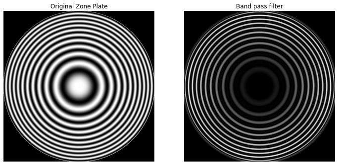
- Bandpass filter
- Credits
Spatial domain and frequency domain filters are commonly classified into four types of filters — low-pass, high-pass, band-reject and band-pass filters. In this article I have notes, code examples and image output for each one of them.
Types of filters
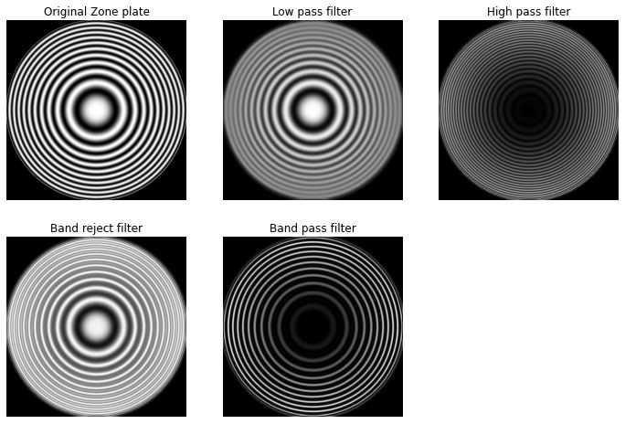
- Lowpass filters: Allow passing only low frequency details, attenuates the high frequency details. Example: Smoothening filters.
- Highpass filters: Allows passing only high frequency details, attenuates the low frequency details. Example: Sharpening mask filters.
- Bandreject filters: Attenuate signal in range of a certain frequency. Allows frequency below a certain threshold and above another threshold to pass.
- Bandpass filters: Only allows signals within a certain band to pass, attenuates the frequencies below a threshold and above another threshold to pass.
Spatial kernels in terms of low-pass kernel — lp(x, y)
| Kernels | Equation |
|---|---|
| Lowpass kernel | lp(x, y) |
| Highpass kernel | hp(x, y) = δ(x, y) - lp(x, y) |
| Bandreject kernel | br(x, y) = lp1(x, y) + hp2(x, y) br(x, y) = lp1(x, y) + (δ(x, y) - lp2(x, y)) |
| Bandpass kernel | bp(x, y) = δ(x, y) - br(x, y) |
δ(x, y)is a unit impulse kernel
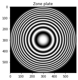
Processing images with these filters using Zone plate
Zone plate is used for testing the characteristics of the filters. There are various versions of zone plates the one I’d be using can be generated with:
Where x, y belong to
[-8.2, 8.2]increasing in steps of0.0275to form a 597x597 image.
def zone(x, y):
    return 0.5 * (1 + math.cos(x * x + y * y))

SIZE = 597
image = np.zeros((SIZE, SIZE))

start = -8.2
end = 8.2
step = 0.0275

def dist_center(y, x):
    global SIZE
    center = SIZE / 2
    return math.sqrt( (x - center)**2 + (y - center)**2)

for y in range(0, SIZE):
    for x in range(0, SIZE):
        if dist_center(y, x) > 300:
            continue
        y_val = start + y * step
        x_val = start + x * step
        image[y, x] = zone(x_val, y_val)
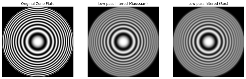
Lowpass filter
kernel_size = 15

lowpass_kernel_gaussian = gkern(kernel_size)
lowpass_kernel_gaussian = lowpass_kernel_gaussian / lowpass_kernel_gaussian.sum()

lowpass_kernel_box = np.ones((kernel_size, kernel_size))
lowpass_kernel_box = lowpass_kernel_box / (kernel_size * kernel_size)

lowpass_image_gaussian = cv2.filter2D(image, -1, lowpass_kernel_gaussian)
lowpass_image_box = cv2.filter2D(image, -1, lowpass_kernel_box)
Highpass filter
In spatial domain, a Highpass filtered image can be obtained by subtracting a Lowpass filtered image from the image itself (like unsharp mask).
highpass_image_gaussian = image - lowpass_image_gaussian
highpass_image_gaussian = np.absolute(highpass_image_gaussian)

highpass_image_box = image - lowpass_image_box
highpass_image_box = np.absolute(highpass_image_box)

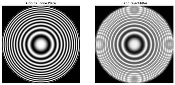
Bandreject filter
Similarly, a Bandreject filtered image can be obtained by adding a Lowpass filtered with a Highpass filtered image (at different threshold).
bandreject_image = lowpass_image_gaussian + highpass_image_box
Bandpass filter
And Bandpass filtered image can be obtained by subtracting the Bandreject filtered image from the image itself.
bandpass_image = image - bandreject_image
bandpass_image = np.absolute(bandpass_image)
Credits
A lot of this is derived from the book Digital Image Processing — by Rafael C. Gonzalez & Richard E. Woods and can be used as quick refresher. I’ll only be listing some key pointers, sample code and the result of running them.

Disclaimer: While I do recommend this book (I use it) for learning digital image processing, if you buy this book via this link — I’ll be paid a certain small percentage in commission.
Want to read more such similar contents?
I like to write articles on topic less covered on internet. They revolve around writing fast algorithms, image processing as well as general software engineering.
I publish many of them on Medium.
If you are already on medium - Please join 4200+ other members and Subscribe to my articles to get updates as I publish.
If you are not on Medium - Medium has millions of amazing articles from 100K+ authors. To get access to those, please join using my referral link. This will give you access to all the benefits of Medium and Medium shall pay me a piece to support my writing!
Thanks!